OpenCV Image Processing (Python)¶

In this exercise, we will gain familiarity with both OpenCV and Python, through a simple 2D image-processing application.

Motivation¶

OpenCV is a mature, stable library for 2D image processing, used in a wide variety of applications. Much of ROS makes use of 3D sensors and point-cloud data, but there are still many applications that use traditional 2D cameras and image processing.

This tutorial uses python to build the image-processing pipeline. Python is a good choice for this application, due to its ease of rapid prototyping and existing bindings to the OpenCV library.

Further Information and Resources¶

Problem Statement¶

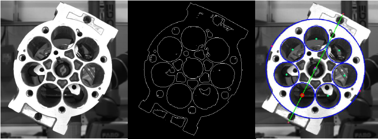
In this exercise, you will create a new node to determine the angular pose of a pump housing using the OpenCV image processing library. The pump’s orientation is computed using a series of processing steps to extract and compare geometry features:

Resize the image (to speed up processing)
Threshold the image (convert to black & white)
Locate the pump’s outer housing (circle-finding)
Locate the piston sleeve locations (blob detection)
Estimate primary axis using bounding box
Determine orientation using piston sleeve locations
Calculate the axis orientation relative to a reference (horizontal) axis

pump images

Implementation¶

Create package¶

This exercise uses a single package that can be placed in any catkin workspace. The examples below will use the ~/catkin_ws workspace from earlier exercises.

Create a new detect_pump package to contain the new python nodes we’ll be making:
```
cd ~/catkin_ws/src
catkin create pkg detect_pump --catkin-deps rospy cv_bridge
```
- all ROS packages depend on rospy
- we’ll use cv_bridge to convert between ROS’s standard Image message and OpenCV’s Image object
- cv_bridge also automatically brings in dependencies on the relevant OpenCV modules
Create a python module for this package:
```
cd detect_pump
mkdir nodes
```
- For a simple package such as this, the Python Style Guide recommends this simplified package structure.
- More complex packages (e.g. with exportable modules, msg/srv defintions, etc.) should us a more complex package structure, with an __init__.py and setup.py.
  - reference Installing Python Scripts
  - reference Handling setup.py

Create an Image Publisher¶

The first node will read in an image from a file and publish it as a ROS Image message on the image topic.

Note: ROS already contains an image_publisher package/node that performs this function, but we will duplicate it here to learn about ROS Publishers in Python.

Create a new python script for our image-publisher node (nodes/image_pub.py). Fill in the following template for a skeleton ROS python node:

#!/usr/bin/env python
import rospy

def start_node():
    rospy.init_node('image_pub')
    rospy.loginfo('image_pub node started')

if __name__ == '__main__':
    try:
        start_node()
    except rospy.ROSInterruptException:
        pass

Allow execution of the new script file:
```
chmod u+x nodes/image_pub.py
```
Build the package and run the image publisher:
```
catkin build
roscore
rosrun detect_pump image_pump.py
```
- You should see the “node started” message
Read the image file to publish, using the filename provided on the command line
1. Import the sys and cv2 (OpenCV) modules:
```
import sys
import cv2
```
2. Pass the command-line argument into the start_node function:
```
def start_node(filename):
...
start_node( rospy.myargv(argv=sys.argv)[1] )
```
  - Note the use of rospy.myargv() to strip out any ROS-specific command-line arguments.
3. In the start_node function, call the OpenCV imread function to read the image. Then use imshow to display it:
```
img = cv2.imread(filename)
cv2.imshow("image", img)
cv2.waitKey(2000)
```
4. Run the node, with the specified image file:
```
rosrun detect_pump image_pub.py ~/industrial_training/exercises/5.4/pump.jpg
```
  - You should see the image displayed
  - Comment out the imshow/waitKey lines, as we won’t need those any more
  - Note that you don’t need to run catkin build after editing the python file, since no compile step is needed.
Convert the image from OpenCV Image object to ROS Image message:
1. Import the CvBridge and Image (ROS message) modules:
```
from cv_bridge import CvBridge
from sensor_msgs.msg import Image
```
2. Add a call to the CvBridge cv2_to_imgmsg method:
```
bridge = CvBridge()
imgMsg = bridge.cv2_to_imgmsg(img, "bgr8")
```

Create a ROS publisher to continually publish the Image message on the image topic. Use a loop with a 1 Hz throttle to publish the message.

pub = rospy.Publisher('image', Image, queue_size=10)
while not rospy.is_shutdown():
    pub.publish(imgMsg)
    rospy.Rate(1.0).sleep()  # 1 Hz

Run the node and inspect the newly-published image message
1. Run the node (as before):
```
rosrun detect_pump image_pub.py ~/industrial_training/exercises/5.4/pump.jpg
```
2. Inspect the message topic using command-line tools:
```
rostopic list
rostopic hz /image
rosnode info /image_pub
```
3. Inspect the published image using the standalone image_view node
```
rosrun image_view image_view
```

Create the Detect_Pump Image-Processing Node¶

The next node will subscribe to the image topic and execute a series of processing steps to identify the pump’s orientation relative to the horizontal image axis.

As before, create a basic ROS python node (detect_pump.py) and set its executable permissions:

#!/usr/bin/env python
import rospy

# known pump geometry
#  - units are pixels (of half-size image)
PUMP_DIAMETER = 360
PISTON_DIAMETER = 90
PISTON_COUNT = 7

def start_node():
    rospy.init_node('detect_pump')
    rospy.loginfo('detect_pump node started')

if __name__ == '__main__':
    try:
        start_node()
    except rospy.ROSInterruptException:
        pass

chmod u+x nodes/detect_pump.py

Note that we don’t have to edit CMakeLists to create new build rules for each script, since python does not need to be compiled.

Add a ROS subscriber to the image topic, to provide the source for images to process.
1. Import the Image message header
```
from sensor_msgs.msg import Image
```
2. Above the start_node function, create an empty callback (process_image) that will be called when a new Image message is received:
```
def process_image(msg):
    try:
       pass
    except Exception as err:
        print err
```
  - The try/except error handling will allow our code to continue running, even if there are errors during the processing pipeline.
3. In the start_node function, create a ROS Subscriber object:
  - subscribe to the image topic, monitoring messages of type Image
  - register the callback function we defined above
```
rospy.Subscriber("image", Image, process_image)
rospy.spin()
```
  - reference: rospy.Subscriber
  - reference: rospy.spin
4. Run the new node and verify that it is subscribing to the topic as expected:
```
rosrun detect_pump detect_pump.py
rosnode info /detect_pump
rqt_graph
```
Convert the incoming Image message to an OpenCV Image object and display it As before, we’ll use the CvBridge module to do the conversion.
1. Import the CvBridge modules:
```
from cv_bridge import CvBridge
```
2. In the process_image callback, add a call to the CvBridge imgmsg_to_cv2 method:
```
# convert sensor_msgs/Image to OpenCV Image
bridge = CvBridge()
orig = bridge.imgmsg_to_cv2(msg, "bgr8")
```
  - This code (and all other image-processing code) should go inside the try block, to ensure that processing errors don’t crash the node.
  - This should replace the placeholder pass command placed in the try block earlier
3. Use the OpenCV imshow method to display the images received. We’ll create a pattern that can be re-used to show the result of each image-processing step.
  1. Import the OpenCV cv2 module:
    import cv2
  2. Add a display helper function above the process_image callback:
    def showImage(img): cv2.imshow('image', img) cv2.waitKey(1)
  3. Copy the received image to a new “drawImg” variable:
    drawImg = orig
  4. Below the except block (outside its scope; at process_image scope, display the drawImg variable:
    # show results showImage(drawImg)
4. Run the node and see the received image displayed.
The first step in the image-processing pipeline is to resize the image, to speed up future processing steps. Add the following code inside the try block, then rerun the node.
```
# resize image (half-size) for easier processing
resized = cv2.resize(orig, None, fx=0.5, fy=0.5)
drawImg = resized
```
- you should see a smaller image being displayed
- reference: resize()
Next, convert the image from color to grayscale. Run the node to check for errors, but the image will still look the same as previously.
```
# convert to single-channel image
gray = cv2.cvtColor(resized, cv2.COLOR_BGR2GRAY)
drawImg = cv2.cvtColor(gray, cv2.COLOR_GRAY2BGR)
```
- Even though the original image looks gray, the JPG file, Image message, and orig OpenCV image are all 3-channel color images.
- Many OpenCV functions operate on individual image channels. Converting an image that appears gray to a “true” 1-channel grayscale image can help avoid confusion further on.
- We convert back to a color image for drawImg so that we can draw colored overlays on top of the image to display the results of later processing steps.
- reference: cvtColor()
Apply a thresholding operation to turn the grayscale image into a binary image. Run the node and see the thresholded image.
```
# threshold grayscale to binary (black & white) image
threshVal = 75
ret,thresh = cv2.threshold(gray, threshVal, 255, cv2.THRESH_BINARY)
drawImg = cv2.cvtColor(thresh, cv2.COLOR_GRAY2BGR)
```
You should experiment with the threshVal paramter to find a value that works best for this image. Valid values for this parameter lie between [0-255], to match the grayscale pixel intensity range. Find a value that clearly highlights the pump face geometry. I found that a value of 150 seemed good to me.
- reference threshold
Detect the outer pump-housing circle.

This is not actually used to detect the pump angle, but serves as a good example of feature detection. In a more complex scene, you could use OpenCV’s Region Of Interest (ROI) feature to limit further processing to only features inside this pump housing circle.
1. Use the HoughCircles method to detect a pump housing of known size:
```
# detect outer pump circle
pumpRadiusRange = ( PUMP_DIAMETER/2-2, PUMP_DIAMETER/2+2)
pumpCircles = cv2.HoughCircles(thresh, cv2.HOUGH_GRADIENT, 1, PUMP_DIAMETER, param2=2, minRadius=pumpRadiusRange[0], maxRadius=pumpRadiusRange[1])
```
  - reference: HoughCircles
2. Add a function to display all detected circles (above the process_image callback):
```
def plotCircles(img, circles, color):
    if circles is None: return

    for (x,y,r) in circles[0]:
        cv2.circle(img, (int(x),int(y)), int(r), color, 2)
```
3. Below the circle-detect, call the display function and check for the expected # of circles (1)
```
plotCircles(drawImg, pumpCircles, (255,0,0))
if (pumpCircles is None):
    raise Exception("No pump circles found!")
elif len(pumpCircles[0])<>1:
    raise Exception("Wrong # of pump circles: found {} expected {}".format(len(pumpCircles[0]),1))
else:
    pumpCircle = pumpCircles[0][0]
```
4. Run the node and see the detected circles.
  - Experiment with adjusting the param2 input to HoughCircles to find a value that seems to work well. This parameter represents the sensitivity of the detector; lower values detect more circles, but also will return more false-positives.
  - Tru removing the min/maxRadius parameters or reducing the minimum distance between circles (4th parameter) to see what other circles are detected.
  - I found that a value of param2=7 seemed to work well
Detect the piston sleeves, using blob detection.

Blob detection analyses the image to identify connected regions (blobs) of similar color. Filtering of the resulting blob features on size, shape, or other characteristics can help identify features of interest. We will be using OpenCV’s SimpleBlobDetector.
1. Add the following code to run blob detection on the binary image:
```
# detect blobs inside pump body
pistonArea = 3.14159 * PISTON_DIAMETER**2 / 4
blobParams = cv2.SimpleBlobDetector_Params()
blobParams.filterByArea = True
blobParams.minArea = 0.80 * pistonArea
blobParams.maxArea = 1.20 * pistonArea
blobDetector = cv2.SimpleBlobDetector_create(blobParams)
blobs = blobDetector.detect(thresh)
```
  - Note the use of an Area filter to select blobs within 20% of the expected piston-sleeve area.
  - By default, the blob detector is configured to detect black blobs on a white background. so no additional color filtering is required.
2. Below the blob detection, call the OpenCV blob display function and check for the expected # of piston sleeves (7):
```
drawImg = cv2.drawKeypoints(drawImg, blobs, (), (0,255,0), cv2.DRAW_MATCHES_FLAGS_DRAW_RICH_KEYPOINTS)
if len(blobs) <> PISTON_COUNT:
    raise Exception("Wring # of pistons: found {} expected {}".format(len(blobs), PISTON_COUNT))
pistonCenters = [(int(b.pt[0]),int(b.pt[1])) for b in blobs]
```
3. Run the node and see if all piston sleeves were properly identified

Detect the primary axis of the pump body.

This axis is used to identify the key piston sleeve feature. We’ll reduce the image to contours (outlines), then find the largest one, fit a rectangular box (rotated for best-fit), and identify the major axis of that box.

Calculate image contours and select the one with the largest area:

# determine primary axis, using largest contour
im2, contours, h = cv2.findContours(thresh, cv2.RETR_TREE, cv2.CHAIN_APPROX_SIMPLE)
maxC = max(contours, key=lambda c: cv2.contourArea(c))

Fit a bounding box to the largest contour:
```
boundRect = cv2.minAreaRect(maxC)
```

Copy these 3 helper functions to calculate the endpoints of the rectangle’s major axis (above the process_image callback):

import math
...

def ptDist(p1, p2):
    dx=p2[0]-p1[0]; dy=p2[1]-p1[1]
    return math.sqrt( dx*dx + dy*dy )

def ptMean(p1, p2):
    return ((int(p1[0]+p2[0])/2, int(p1[1]+p2[1])/2))

def rect2centerline(rect):
    p0=rect[0]; p1=rect[1]; p2=rect[2]; p3=rect[3];
    width=ptDist(p0,p1); height=ptDist(p1,p2);

    # centerline lies along longest median
    if (height > width):
        cl = ( ptMean(p0,p1), ptMean(p2,p3) )
    else:
        cl = ( ptMean(p1,p2), ptMean(p3,p0) )

    return cl

Call the rect2centerline function from above, with the bounding rectangle calculated earlier. Draw the centerline on top of our display image.
```
centerline = rect2centerline(cv2.boxPoints(boundRect))
cv2.line(drawImg, centerline[0], centerline[1], (0,0,255))
```

The final step is to identify the key piston sleeve (closest to centerline) and use position to calculate the pump angle.

Add a helper function to calculate the distance between a point and the centerline:

def ptLineDist(pt, line):
    x0=pt[0]; x1=line[0][0]; x2=line[1][0];
    y0=pt[1]; y1=line[0][1]; y2=line[1][1];
    return abs((x2-x1)*(y1-y0)-(x1-x0)*(y2-y1))/(math.sqrt((x2-x1)*(x2-x1)+(y2-y1)*(y2-y1)))

Call the ptLineDist function to find which piston blob is closest to the centerline. Update the drawImg to show which blob was identified.

# find closest piston to primary axis
closestPiston = min( pistonCenters, key=lambda ctr: ptLineDist(ctr, centerline))
cv2.circle(drawImg, closestPiston, 5, (255,255,0), -1)

Calculate the angle between the 3 key points: piston sleeve centerpoint, pump center, and an arbitrary point along the horizontal axis (our reference “zero” position).

Add a helper function findAngle to calculate the angle between 3 points:

import numpy as np

def findAngle(p1, p2, p3):
    p1=np.array(p1); p2=np.array(p2); p3=np.array(p3);
    v1=p1-p2; v2=p3-p2;
    return math.atan2(-v1[0]*v2[1]+v1[1]*v2[0],v1[0]*v2[0]+v1[1]*v2[1]) * 180/3.14159

Call the findAngle function with the appropriate 3 keypoints:

# calculate pump angle
p1 = (orig.shape[1], pumpCircle[1])
p2 = (pumpCircle[0], pumpCircle[1])
p3 = (closestPiston[0], closestPiston[1])
angle = findAngle(p1, p2, p3)
print "Found pump angle: {}".format(angle)

You’re done! Run the node as before. The reported pump angle should be near 24 degrees.

Challenge Exercises¶

For a greater challenge, try the following suggestions to modify the operation of this image-processing example:

Modify the image_pub node to rotate the image by 10 degrees between each publishing step. The following code can be used to rotate an image:

def rotateImg(img, angle):
    rows,cols,ch = img.shape
    M = cv2.getRotationMatrix2D((cols/2,rows/2),angle,1)
    return cv2.warpAffine(img,M,(cols,rows))

Change the detect_pump node to provide a service that performs the image detection. Define a custom service type that takes an input image and outputs the pump angle. Create a new application node that subscribes to the image topic and calls the detect_pump service.
Try using HoughCircles instead of BlobDetector to locate the piston sleeves.